PointNet++:Aggregate Local Features with Sampling And Grouping

Review of PointNet

One of the most prominent shortcomings of PointNet is that PointNet does not capture local structures induced by the metric space points live in, because PointNet only extract features on single point, or use max pool to aggregate global points. This limits its ability to recognize fine-grained patterns and generalizability to complex scenes and has led to the poor performance of PointNet in segmentation, especially in partial segmentation scenarios.

PointNet++

Fig.1 Overrall of PointNet++

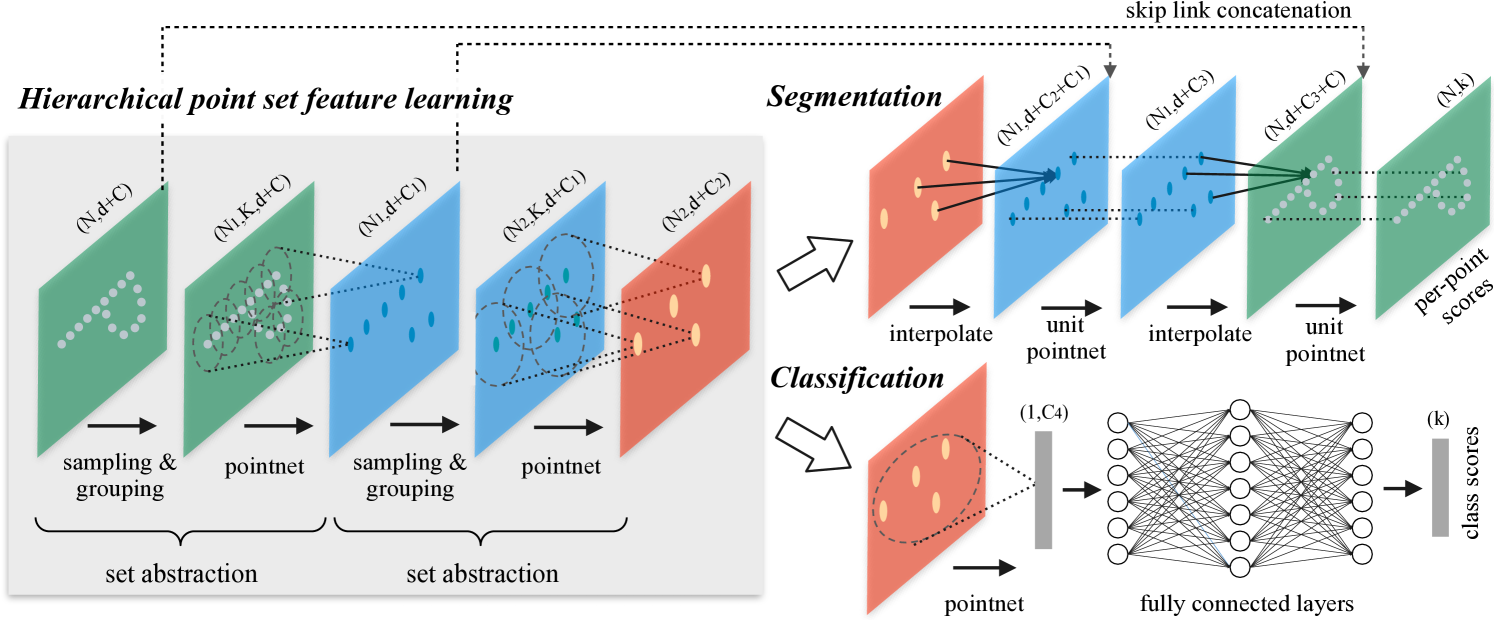
Figure 2: Illustration of our hierarchical feature learning architecture and its application for set
segmentation and classification using points in 2D Euclidean space as an example. Single scale point
grouping is visualized here. For details on density adaptive grouping, see Fig. 3

While PointNet uses a single max pooling operation to aggregate the whole point set, PointNet++ builds a hierarchical grouping of points and progressively abstract larger and larger local regions along the hierarchy based on CNNs. As show in Fig.1, the whole PointNeet++ can be divided into three parts, set abstraction, classification and segmentation. Here we mainly discuss set abstraction and segmentation (as classification is nearly the same as that in PointNet).

Set abstraction

The set abstraction level is made of three key layers: Sampling layer, Grouping layer and PointNet layer. The Sampling layer selects a set of points from input points use FPS, which defines the centroids of local regions. Grouping layer then constructs local region sets by finding “neighboring” points around the centroids. PointNet layer uses a mini-PointNet to encode local region patterns into feature vectors. A set abstraction level takes an $N\times(d + C)$ tensot as input that is from $N$ points with d-dim coordinates and C-dim point feature. It outputs an $N’\times (d + C’ )$ tensor of $N’$ subsampled points with d-dim coordinates and new $C’$-dim feature vectors summarizing local context.

Here’s the code of this layer:

class PointNetSetAbstraction(nn.Module):
    def __init__(self, npoint, radius, nsample, in_channel, mlp, group_all):
        super(PointNetSetAbstraction, self).__init__()
        self.npoint = npoint
        self.radius = radius
        self.nsample = nsample
        self.mlp_convs = nn.ModuleList()
        self.mlp_bns = nn.ModuleList()
        last_channel = in_channel
        for out_channel in mlp:
            self.mlp_convs.append(nn.Conv2d(last_channel, out_channel, 1))
            self.mlp_bns.append(nn.BatchNorm2d(out_channel))
            last_channel = out_channel
        self.group_all = group_all

    def forward(self, xyz, points):
        """
        Input:
            xyz: input points position data, [B, C, N]
            points: input points data, [B, D, N]
        Return:
            new_xyz: sampled points position data, [B, C, S]
            new_points_concat: sample points feature data, [B, D', S]
        """
        xyz = xyz.permute(0, 2, 1)
        if points is not None:
            points = points.permute(0, 2, 1)

        if self.group_all:
            new_xyz, new_points = sample_and_group_all(xyz, points)
        else:
            new_xyz, new_points = sample_and_group(self.npoint, self.radius, self.nsample, xyz, points)
        # new_xyz: sampled points position data, [B, npoint, C]
        # new_points: sampled points data, [B, npoint, nsample, C+D]
        new_points = new_points.permute(0, 3, 2, 1) # [B, C+D, nsample,npoint]
        for i, conv in enumerate(self.mlp_convs):
            bn = self.mlp_bns[i]
            new_points =  F.relu(bn(conv(new_points)))

        new_points = torch.max(new_points, 2)[0]
        new_xyz = new_xyz.permute(0, 2, 1)
        return new_xyz, new_points

Grouping layer

The input to this layer is a point set of size $N\times(d + C)$ and the coordinates of a set of centroids of size $N’\times d$. The output are groups of point sets of size $N’\times K \times (d + C)$, where each group corresponds to a local region and $K$ is the number of points sambled by ball query or kNN in the neighborhood of centroid points. Ball query finds all points that are within a radius to the query point (an upper limit of $K$ is set in implementation, if number of points is less than $K$, resample the centroid point). Compared with kNN, ball query’s local neighborhood guarantees a fixed region scale thus making local region feature more generalizable across space, which is preferred for tasks requiring local pattern recognition. $K$ varies across groups but the succeeding PointNet layer is able to convert flexible number of points into a fixed length local region feature vector.

Here’s the code of ball query:

def query_ball_point(radius, nsample, xyz, new_xyz):
    """
    Input:
        radius: local region radius
        nsample: max sample number in local region
        xyz: all points, [B, N, 3]
        new_xyz: query points, [B, S, 3]
    Return:
        group_idx: grouped points index, [B, S, nsample]
    """
    device = xyz.device
    B, N, C = xyz.shape
    _, S, _ = new_xyz.shape
    group_idx = torch.arange(N, dtype=torch.long).to(device).view(1, 1, N).repeat([B, S, 1])
    sqrdists = square_distance(new_xyz, xyz)
    group_idx[sqrdists > radius ** 2] = N
    group_idx = group_idx.sort(dim=-1)[0][:, :, :nsample]
    group_first = group_idx[:, :, 0].view(B, S, 1).repeat([1, 1, nsample])
    mask = group_idx == N
    group_idx[mask] = group_first[mask]
    return group_idx

PointNet layer

In this layer, the input are $N’$ local regions of points with data size $N’\times K \times (d + C)$. Each local region in the output is abstracted by its centroid and local feature that encodes the centroid’s neighborhood. Output data size is $N’\times K \times (d + C’)$. The coordinates of points in a local region are firstly translated into a local frame relative to the centroid point: $x^{(j)}_i = x^{(j)}_i - \hat{x}^{(j)}$ for $i = 1, 2, …, K$ and $j = 1, 2, …, d$ where $\hat{x}$ is the coordinate of the centroid. By using relative coordinates together with point features we can capture point-to-point relations in the local region.

MSG and MRG

Fig.2 MSG and MRG

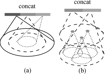
Figure 3: (a) Multi-scale cross-level adaptive scale selection grouping (MSG); (b) Multiresolution grouping (MRG).

In the paper, the author conducted a comparative experiment to address the issue of PointNet’s poor performance on uneven point clouds. They used the original PointNet++ and found that its performance was not as good as PointNet in point clouds with uneven density. To improve the performance, PointNet++ introduces two solutions: Multi-Scale Grouping (MSG) and Multi-Resolution Grouping (MRG).

MSG uses multiple scales (radius) in each grouping layer to determine the range of the domain, and each range is extracted from the PointNet layer feature and then integrated to obtain a new multi-scale feature.But due to compute for serveral times, the MSG approach is computationally expensive.

Each feature of MRG consists of two parts: the features obtained by PointNet layer in the domain of this layer, and the features obtained by PointNet layer in the domain of the previous layer. When the point cloud density is uneven, different weights can be given to the left and right feature vectors by judging the point cloud density of the current patch. For example, when the density in the patch is too small, the points contained in the left eigenvector are more sparse, which is easily affected by undersampling, so the weight of the right eigenvector is increased.

Fig.3 Exprements on MSG and MRG

Figure 4: Left: Point cloud with random point dropout. Right: Curve showing advantage of our density adaptive strategy in dealing with non-uniform density. DP means random input dropout during training; otherwise training is on uniformly dense points. See Sec.3.3 for details.

It can be seen that MSG and MRG have no improvement in classification accuracy compared with SSG (single-scale), but when the point cloud is very sparse, using MSG can maintain good robustness. Random input dropout (DP) also greatly improves the robustness.

Segmentation

PointNet++ adopts a hierarchical propagation strategy with distance based interpolation and across level skip links. In a feature propagation level, PointNet++ propagates point features from $N_l \times (d + C)$ points to $N_{l-1}$ points where $N_{l-1}$ and $N_l$ (with $N_l \leq N_{l-1}$) are point set size of input and output of set abstraction level $l$. PointNet++ achieves feature propagation by interpolating feature values $f$ of $N_l$ points at coordinates of the $N_{l-1}$ points. Among the many choices for interpolation, PointNet++ uses inverse distance weighted average based on k nearest neighbors (as in following equation, in default $p = 2, k = 3$). The interpolated features on $N_{l-1}$ points are then concatenated with skip linked point features from the set abstraction level. Then the concatenated features are passed through a “unit pointnet”, which is similar to one-by-one convolution in CNNs. A few shared fully connected and ReLU layers are applied to update each point’s feature vector. The process is repeated until we have propagated features to the original set of points.
$$
f^{(j)}(x)=\frac{\sum_{i=1}^kw_i(x)f_i^{(i)}}{\sum_{i=1}^kw_i(x)}\quad\text{where}\quad w_i(x)=\frac{1}{d(x, x_i)^p}, j=1,2,…,C
$$

Here’s the code:

class PointNetFeaturePropagation(nn.Module):
    def __init__(self, in_channel, mlp):
        super(PointNetFeaturePropagation, self).__init__()
        self.mlp_convs = nn.ModuleList()
        self.mlp_bns = nn.ModuleList()
        last_channel = in_channel
        for out_channel in mlp:
            self.mlp_convs.append(nn.Conv1d(last_channel, out_channel, 1))
            self.mlp_bns.append(nn.BatchNorm1d(out_channel))
            last_channel = out_channel

    def forward(self, xyz1, xyz2, points1, points2):
        """
        Input:
            xyz1: input points position data, [B, C, N]
            xyz2: sampled input points position data, [B, C, S]
            points1: input points data, [B, D, N]
            points2: input points data, [B, D, S]
        Return:
            new_points: upsampled points data, [B, D', N]
        """
        xyz1 = xyz1.permute(0, 2, 1)
        xyz2 = xyz2.permute(0, 2, 1)

        points2 = points2.permute(0, 2, 1)
        B, N, C = xyz1.shape
        _, S, _ = xyz2.shape

        if S == 1:
            interpolated_points = points2.repeat(1, N, 1)
        else:
            dists = square_distance(xyz1, xyz2)
            dists, idx = dists.sort(dim=-1)
            dists, idx = dists[:, :, :3], idx[:, :, :3]  # [B, N, 3]

            dist_recip = 1.0 / (dists + 1e-8)
            norm = torch.sum(dist_recip, dim=2, keepdim=True)
            weight = dist_recip / norm
            interpolated_points = torch.sum(index_points(points2, idx) * weight.view(B, N, 3, 1), dim=2)

        if points1 is not None:
            points1 = points1.permute(0, 2, 1)
            new_points = torch.cat([points1, interpolated_points], dim=-1)
        else:
            new_points = interpolated_points

        new_points = new_points.permute(0, 2, 1)
        for i, conv in enumerate(self.mlp_convs):
            bn = self.mlp_bns[i]
            new_points = F.relu(bn(conv(new_points)))
        return new_points

Reference

1. Charles Ruizhongtai Qi, Li Yi, Hao Su, and Leonidas J. Guibas. Pointnet++: Deep hierarchical feature learning on point sets in a metric space. In NIPS, 2017. ↩
2. Pytorch_Pointnet_Pointnet2 ↩