Generative Adverserial Networks

Architecture

Fig.1 GAN Architecture

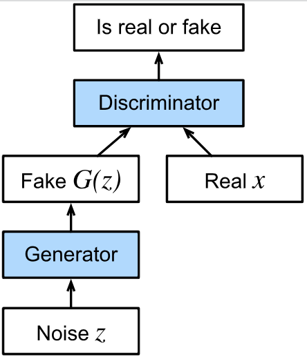
The GAN architecture is illustrated in Fig.1 . There are two pieces in GAN architecture —— a generator and a discriminator. The generator is used to generate objects that need to be generated from the latent space The discriminator attempts to distinguish fake and real data from each other. Both networks are in competition with each other. The generator network attempts to fool the discriminator network. At that point, the discriminator network adapts to the new fake data. This information, in turn is used to improve the generator network, and so on.

Idea

The discriminator is a binary classifier to distinguish if the input is real (from real data) or fake (from the generator). Typically, the discriminator outputs a scalar prediction $o\in \mathbb{R}$ for input $\textbf{x}$, such as using a fully connected layer with hidden size 1, and then applies sigmoid function to obtain the predicted probability $D(\textbf{x}) = \frac{1}{1+e^{-o}}$ . Assume the label $y$ for the true data is 1 and 0 for the fake data. Train the discriminator to minimize the cross-entropy loss.

$$
\min\limits_{D}{-y\log{D(\textbf{x})} - (1-y)\log{(1-D(\textbf{x}))} }
$$

For the generator, it first draws some parameter $\textbf{z}\in \mathbb{R}^d$ from a source of randomness, for example, a normal distribution. It then applies a function to generate $x’=G(\textbf{z})$. The goal of the generator is to fool the discriminator to classify $x’=G(\textbf{z})$ as true data $D(G(\textbf{z}))\approx 1$. In other words, for a given discriminator $D$, update the parameters of the generator $G$ to maximize the cross-entropy loss when $y=0$.

$$
\max\limits_{G}{-(1-y)\log{(1-D(G(\textbf{z})))}}=\max\limits_{G}{-\log{(1-D(G(\textbf{z})))}}
$$

If the generator does a perfect job, then $D(\textbf{x}’)\approx 1$ , so the above loss is near 0, which results in the gradients that are too small to make good progress for the discriminator. So commonly, minimize the following loss:

$$
\min\limits_{G}{-y\log{D(G(\textbf{z}))}}=\min\limits_{G}{-\log{D(G(\textbf{z}))}}
$$

which is just feeding $x’=G(\textbf{z})$ into the discriminator but giving label $y=1$.

To sum up $G$, and $D$ are playing a “minimax” game with the comprehensive objective function:
$$
\min\limits_{D}\max\limits_{D}{ -E_{\text{x$\sim$Data}}\log{D(\textbf{x})}-E_{\text{z$\sim$Noise}}\log{(1-D(G(\textbf{z})))} }
$$

Procedure

Fig.2 Training Procedure

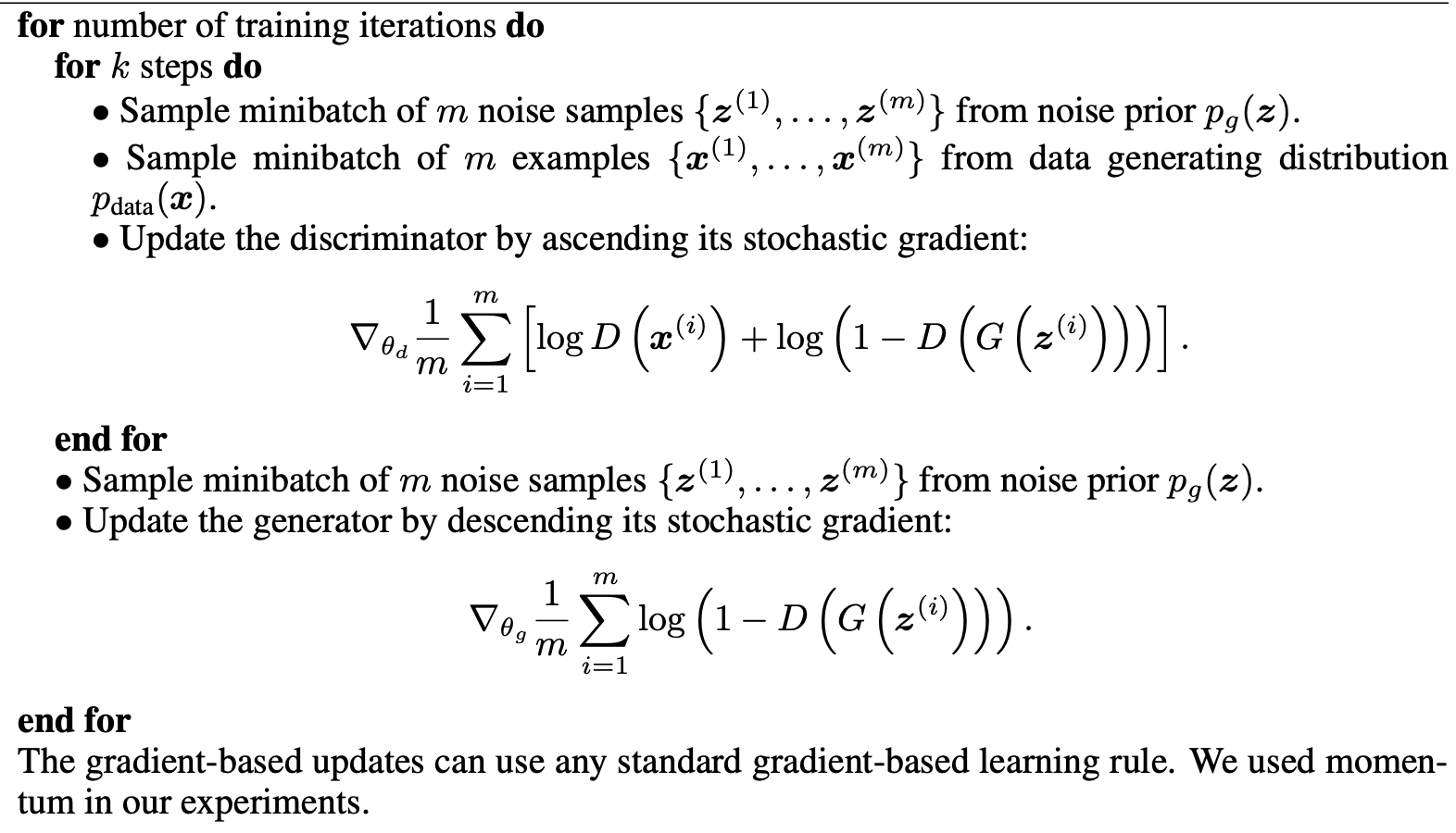
See Fig.2, GAN are trained by simultaneously updating the discriminative distribution ($D$, blue, dashed line) so that it discriminates between samples from the data generating distribution (black, dotted line) $p_{x}$ from those of the generative distribution $p_g (G)$ (green, solid line). The lower horizontal line is the domain from which $\textbf{z}$ is sampled, in this case uniformly. The horizontal line above is part of the domain of $\textbf{x}$. The upward arrows show how the mapping $\textbf{x} = G(\textbf{z})$ imposes the non-uniform distribution $p_g$ on transformed samples. $G$ contracts in regions of high density and expands in regions of low density of $p_g$. (a) Consider an adversarial pair near convergence: $p_g$ is similar to $p_{data}$ and $D$ is a partially accurate classifier. (b) In the inner loop of the algorithm $D$ is trained to discriminate samples from data, converging to $D^{∗}(\textbf{x}) =\frac{p_{data}(\textbf{x})}{p_{data}(\textbf{x})+p_g(\textbf{x})}$ . (c) After an update to $G$, gradient of $D$ has guided $G(\textbf{z})$ to flow to regions that are more likely to be classified as data. (d) After several steps of training, if $G$ and $D$ have enough capacity, they will reach a point at which both cannot improve because $p_g = p_{data}$. The discriminator is unable to differentiate between the two distributions, i.e. $D(\textbf{x}) = \frac{1}{2}$.

Pytorch Implementation

def train(G, D, dataloader, optimizer_G, optimizer_D, latent_dim, epochs):
    loss = nn.BCELoss()
    for epoch in range(epochs):
        for real, _ in dataloader:
            batch_size = real.shape[0]
            REAL = torch.ones(batch_size, 1))
            FAKE = torch.zeros(batch_size, 1))
            z = torch.normal(0, 1, size=(batch_size, latent_dim))
            fake = G(z)

            loss_d = (loss(D(real), REAL) + loss(D(fake.detach()), FAKE) / 2
            optimizer_D.zero_grad()
            loss_d.backward()
            optimizer_D.step()

            loss_g = loss(D(fake), REAL)
            optimizer_G.zero_grad()
            loss_g.backward()
            optimizer_G.step()

Reference

1. Goodfellow, I.J., Pouget-Abadie, J., Mirza, M., Xu, B., Warde-Farley, D., Ozair, S., Courville, A.C., & Bengio, Y. (2014). Generative Adversarial Nets. NIPS. ↩
2. Journal of Machine Learning Research 21 (23), 1-7, 2020. 183, 2020. Dive into deep learning. 2020. A Zhang, ZC Lipton, M Li, AJ Smola. ↩