HiFA

Abstract

The advancements in automatic text-to-3D generation have been remarkable. Most existing methods use pre-trained text-to-image diffusion models to optimize 3D representations like Neural Radiance Fields (NeRFs) via latent-space denoising score matching. Yet, these methods often result in artifacts and inconsistencies across different views due to their suboptimal optimization approaches and limited understanding of 3D geometry. Moreover, the inherent constraints of NeRFs in rendering crisp geometry and stable textures usually lead to a two-stage optimization to attain high-resolution details. This work proposes holistic sampling and smoothing approaches to achieve high-quality text-to-3D generation, all in a single-stage optimization. We compute denoising scores in the text-to-image diffusion model’s latent and image spaces. Instead of randomly sampling timesteps (also referred to as noise levels in denoising score matching), we introduce a novel timestep annealing approach that progressively reduces the sampled timestep throughout optimization. To generate high-quality renderings in a single-stage optimization, we propose regularization for the variance of z-coordinates along NeRF rays. To address texture flickering issues in NeRFs, we introduce a kernel smoothing technique that refines importance sampling weights coarse-to-fine, ensuring accurate and thorough sampling in high-density regions. Extensive experiments demonstrate the superiority of our method over previous approaches, enabling the generation of highly detailed and view-consistent 3D assets through a single-stage training process.

Overview

Fig.1 HiFA

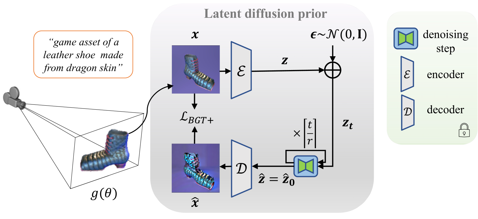
Overview of our proposed method for text-to-3D synthesis. We aim to optimize a 3D model $g(θ)$ using a pre-trained 2D latent diffusion prior. To achieve this, we employ a latent diffusion model to provide gradients. Specifically, the diffusion model takes a rendered image $x$ as input and provides the estimate of the input rendered image, denoted as $\hat{x}$. Unlike existing works that solely focus on computing noise residuals in the low-resolution latent space of the diffusion model, we propose a novel loss $\mathcal{L}_{\text{BGT+}}$ that computes a higherresolution image residual.

Advancing Training Process with Reformulated SDS

The SDS gradient in the latent space of SD is written as

$$
\nabla _{\theta}\mathcal{L}_{\text{SDS}}(\phi, {\bf z}) = \mathbb{E}_{t, {\epsilon}}[\omega(t)(\hat{\epsilon} - \epsilon) \frac{\partial {\bf z}}{\partial \theta} ]
$$

which performs the diffusion process in the latent space, resulting in changes to the SDS gradients in this scenario.

A specific formulation for SDS can be formulated as

\begin{aligned} \displaystyle\mathcal{L}_{\text{SDS}}(\phi,{\bf z})& =\mathbb{E}_{t,{\bf {\epsilon}}}[\omega(t)\frac{\sqrt{\bar{\alpha}_{t}}}{2\sqrt{1-\bar{\alpha}_{t}}}\|{\bf z}-\hat{\bf z}_{\text{1step}}\|^{2}],\text{where} \\ & \displaystyle\hat{\bf z}_{\text{1step}}=\frac{1}{\sqrt{\bar{\alpha}_{t}}}({\bf z}_{t}-\sqrt{1-\bar{\alpha}_{t}}\epsilon_{\phi}({\bf z}_{t};{\bf y},t)) \end{aligned}

with the proof

\begin{aligned} \displaystyle\nabla_{\theta}\mathcal{L}_{\text{SDS}}(\phi,{\bf z}) = & \displaystyle\quad\omega(t)\frac{\sqrt{\bar{\alpha}_{t}}}{\sqrt{1-\bar{\alpha}_{t}}}({\bf z}-\hat{\bf z}_{\text{1step}})\frac{\partial{\bf z}}{\partial\theta} \\ = & \displaystyle\quad\omega(t)\frac{\sqrt{\bar{\alpha}_{t}}}{\sqrt{1-\bar{\alpha}_{t}}}({\bf z}-\frac{1}{\sqrt{\bar{\alpha}_{t}}}({\bf z}_{t}-\sqrt{1-\bar{\alpha}_{t}}\epsilon_{\phi}({\bf z}_{t};{\bf y},t)))\frac{\partial{\bf z}}{\partial\theta} \\ = & \displaystyle\quad\omega(t)\frac{\sqrt{\bar{\alpha}_{t}}}{\sqrt{1-\bar{\alpha}_{t}}}(\frac{\sqrt{1-\bar{\alpha}_{t}}}{\sqrt{\bar{\alpha}_{t}}}(\hat{\bf {\epsilon}}-{\bf \epsilon}))\frac{\partial z}{\partial\theta} \\ = & \displaystyle\quad\omega(t)(\hat{\bf {\epsilon}}-{\bf \epsilon})\frac{\partial{\bf z}}{\partial\theta} \end{aligned}

where $\hat{\bf z}_{\text{1step}}$ is the denoised $\hat{\bf z}$ estimate. To address OOD issue of the diffusion input and divergence issue of the diffusion output, HiFA employs a more accurate estimation for the latent vector ${\bf z}$, which is denoted as $\hat{\bf z}$, obtained through iterative denoisinginstead of using $\hat{\bf z}_{\text{1step}}$ for SDS, and gradually decreases the intensity of the added noise during training by annealing the step $t$. Thus, this adapted loss is
denoted as $\mathcal{L}_{\text{BGT}}$, formally written as

$$
\mathcal{L}_{\text{BGT}}(\phi,\mathbf{z},\mathbf{\hat{z}})=\mathbb{E}_{t,\mathbf{\epsilon}}||\mathbf{\mathbf{z}-\hat{z}}||^{2}
$$

After obtaining the estimated latent vector $\hat{\bf z}$, a further adapted loss $\mathcal{L}_{\text{BGT+}}$ can be naturally obtained, by incorporating additional supervision for recovered images

$$
\mathcal{L}_{\text{BGT+}}(\phi,\mathbf{z},\mathbf{\hat{z}})=\mathbb{E}_{t,\mathbf{\epsilon}}[||\mathbf{\mathbf{z}-\hat{z}}||^{2}+\lambda_{\text{rgb}}||\mathbf{\mathbf{x}-\hat{x}}||^{2}]
$$

$\lambda_{\text{rgb}}$ is a scaling parameter. The time step $t$ is scheduled by

$$
t = t_{\max} - (t_{\max} - t_{\min})\sqrt{\frac{\text{iter}}{\text{total_iter}}}
$$

where $t$ decreases rapidly at the beginning of the training process and slows down toward the end. This scheduling strategy allocates more training steps to lower values of $t$, ensuring that fine-grained details can be adequately learned during the latter stages of training.

Advanced supervision for NeRFs

Fig.2 Illustration of the depth loss $\mathcal{L}_d$

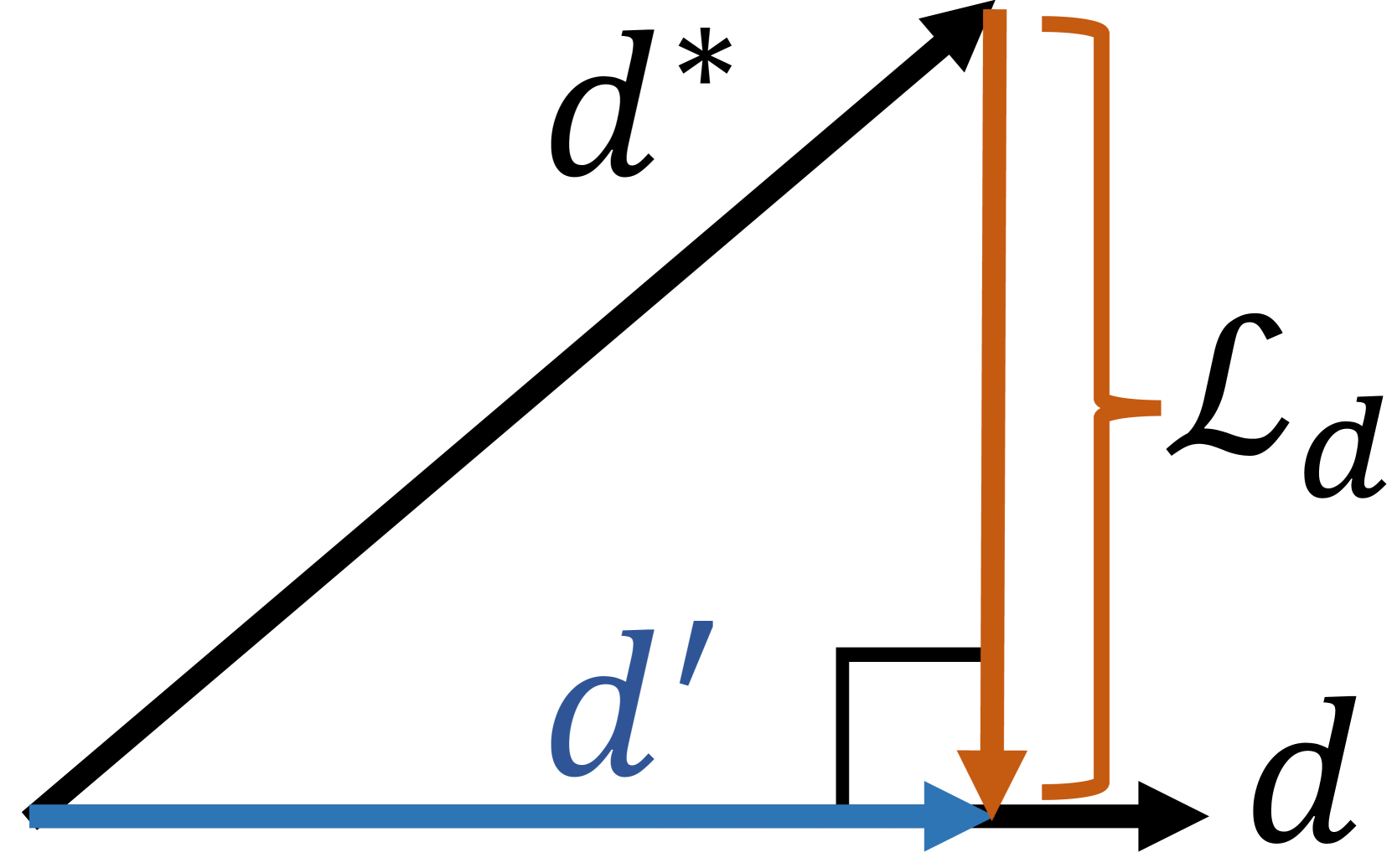
A regularization loss $\mathcal{L}_{d}$ on the disparity map ${\bf d}$ is leveraged to ensure multi-view consistency with a pre-trained depth predictor to estimate the pseudo ground truth of the disparity map ${\bf d}^*$

\begin{aligned} \mathbf{d}^{\prime}=\frac{\langle\mathbf{d},\mathbf{d}^{*}\rangle\mathbf{d}}{\|\mathbf{d}\|^{2}}\text{, and }\mathcal{L}_{d}=\mathbb{E}_{\mathbf{d}}\|\mathbf{d}^{\prime}-\mathbf{d}^{*}\|^{2} \end{aligned}

To reduce the variance of the distribution of the sampled z-coordinates ${z}_i$ along the ray $r$, HiFA computes the z-variance along thecray $r$, denoted as $\sigma^{2}_{z_{r}}$

$$
\sigma^{2}_{z_{r}}=\mathbb{E}_{z_{i}}[(z_{i}-\mu_{z_{r}})^{2}]=\sum_{i}(z_{i}-\mu_{z_{r}})^{2}\frac{w_{i}}{\sum_{i}w_{i}}
$$

The regularization loss $\mathcal{L}_{\text{zvar}}$ for the variance $\sigma^{2}_{z_{r}}$ is defined as

$$
\mathcal{L}_{\text{zvar}}=\mathbb{E}_{r}\delta_{r}\sigma^{2}_{z_{r}}\quad \delta_{r}=1\text{ if }\sum_{i}w_{i}>0.5,\text{ else }0
$$

and the total loss function is

$$
\mathcal{L}=\quad\mathcal{L}_{\text{BGT+}}+\lambda_{d}\mathcal{L}_{d}+\lambda_{\text{zvar}}\mathcal{L}_{\text{zvar}}
$$

Reference

1. Zhu, J., & Zhuang, P. (2023). HiFA: High-fidelity Text-to-3D with Advanced Diffusion Guidance. ArXiv, abs/2305.18766. ↩