3D Gaussian Splatting

Abstract

Radiance Field methods have recently revolutionized novel-view synthesis of scenes captured with multiple photos or videos. However, achieving high visual quality still requires neural networks that are costly to train and render, while recent faster methods inevitably trade off speed for quality. For unbounded and complete scenes (rather than isolated objects) and 1080p resolution rendering, no current method can achieve real-time display rates. We introduce three key elements that allow us to achieve state-of-the-art visual quality while maintaining competitive training times and importantly allow high-quality real-time ( ≥ 30 fps) novel-view synthesis at 1080p resolution. First, starting from sparse points produced during camera calibration, we represent the scene with 3D Gaussians that preserve desirable properties of continuous volumetric radiance fields for scene optimization while avoiding unnecessary computation in empty space; Second, we perform interleaved optimization/density control of the 3D Gaussians, notably optimizing anisotropic covariance to achieve an accurate representation of the scene; Third, we develop a fast visibility-aware rendering algorithm that supports anisotropic splatting and both accelerates training and allows real-time rendering. We demonstrate state-of-the-art visual quality and real-time rendering on several established datasets.

Overview

Fig.1 Overview

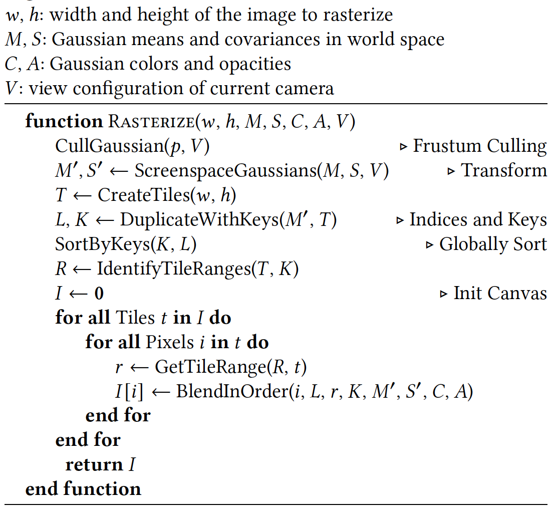
Optimization starts with the sparse SfM point cloud and creates a set of 3D Gaussians. We then optimize and adaptively control the density of this set of Gaussians. During optimization we use our fast tile-based renderer, allowing competitive training times compared to SOTA fast radiance field methods. Once trained, our renderer allows real-time navigation for a wide variety of scenes.

Starting from a set of images of a static scene together with the corresponding cameras calibrated by SfM which produces a sparse point cloud as a sideeffect, a set of 3D Gaussians that allows a very flexible optimization regime is defined by a position (mean), covariance matrix and opacity $\alpha$. This results in a reasonably compact representation of the 3D scene, in part because highly anisotropic volumetric splats can be used to represent fine structures compactly. The directional appearance component (color) of the radiance field is represented via spherical harmonics (SH), following standard practice. The algorithm proceeds to create the radiance field representation via a sequence of optimization steps of 3D Gaussian parameters, i.e., position, covariance, $\alpha$ and SH coefficients interleaved with operations for adaptive control of the Gaussian density. The key to the efficiency is the tile-based rasterizer that allows $\alpha$-blending of anisotropic splats, respecting visibility order thanks to fast sortingand a fast backward pass by tracking accumulated $\alpha$ values, without a limit on the number of Gaussians that can receive gradients.

Point-Based Rendering and Radiance Fields

Point-based $\alpha$-blending and NeRF-style volumetric rendering share essentially the same image formation model. Specifically, the color $C$ is given by volumetric rendering along a ray:

$$
C=\sum_{i=1}^{N}T_{i}(1-\exp(-\sigma_{i}\delta_{i}))\mathbf{c}_{i}\hskip 5.0pt\text{ with }\hskip 5.0ptT_{i}=\exp\left(-\sum_{j=1}^{i-1}\sigma_{j}\delta_{j}\right)
$$

where samples of density $\sigma$, transmittance $T$ , and color $\mathbf{c}$ are taken along the ray with intervals $\delta_i$ . This can be re-written as

$$
C=\sum_{i=1}^{N}T_{i}\alpha_{i}\mathbf{c}_{i}
$$

with

$$
\alpha_{i}=(1-\exp(-\sigma_{i}\delta_{i}))\hskip 5.0pt\text{and}\hskip 5.0ptT_{i}=\prod_{j=1}^{i-1}(1-\alpha_{i})
$$

A typical neural point-based approach computes the color $C$ of a pixel by blending $\mathcal{N}$ ordered points overlapping the pixel

$$
C=\sum_{i\in\mathcal{N}}\mathbf{c}_{i}\alpha_{i}\prod_{j=1}^{i-1}(1-\alpha_{j})
$$

where $\mathbf{c}_i$ is the color of each point and $\alpha_i$ is given by evaluating a 2D Gaussian with covariance $\Sigma$ multiplied with a learned per-point opacity.

Although the image formation model is the same, the rendering algorithm is very different. NeRFs are a continuous representation implicitly representing empty/occupied space; expensive random sampling is required to find the samples with consequent noise and computational expense. In contrast, points are an unstructured, discrete representation that is flexible enough to allow creation, destruction, and displacement of geometry similar to NeRF. This is achieved by optimizing opacity and positions, while avoiding the shortcomings of a full volumetric representation.

Differentiable 3D Gaussian Splatting

The 3D Gaussians are defined by a full 3D covariance matrix $\Sigma$ defined in world space centered at point (mean) $\mu$ and then multiplied by $\alpha$ in blending process.

$$
G(x) = e^{-\frac{1}{2}(x)^T\Sigma ^{-1}(x)}
$$

To project the 3D Gaussians to 2D for rendering, given a viewing transformation $W$, the covariance matrix $\Sigma^{\prime}$ in camera coordinates is given as follows

$$
\Sigma^{\prime} = JW\Sigma W^TJ^T
$$

where $J$ is the Jacobian of the affine approximation of the projective transformation. As Gradient descent cannot be easily constrained to produce valid covariance matrices which have physical meaning only when they are positive semi-definite, given a scaling matrix $S$ and rotation matrix $R$, the corresponding $\Sigma$ is defined as

$$
\Sigma = RSS^TR^T
$$

To allow independent optimization of both factors, $S$ and $R$ are stored separately: a 3D vector $s$ for scaling and a quaternion $q$ to represent rotation. These can be trivially converted to their respective matrices and combined, making sure to normalize $q$ to obtain a valid unit quaternion.

Fast Differentiable Rasterizer for Gaussians

Fig.2 GPU software rasterization of 3D Gaussians

1. Divide the entire image into $16\times 16$ tiles, and select 3D Gaussians that are visible and have a confidence over 0.99 in each tile’s view frustum.
2. Assign a key for each splats instance with up to 64 bits where the lower 32 bits encode its projected depth and the higher bits encode the index of the overlapped tile.
3. Sort Gaussian splats by key to get the Gaussian list of each tile.
4. Start a thread block for each tile. Each thread block first cooperatively loads the of Gaussian splats into shared memory, and then for a given pixel, accumulates the color and value by traversing the list from front to back.
5. When the preset saturation is reached in a pixel (i.e. equal to 1), the corresponding thread stops running.
6. At regular intervals, threads in the tile are queried, and processing of the entire tile is terminated when all pixels are saturated (i.e. become 1).

Optimization with Adaptive Density Control of 3D Gaussians

Adaptive Control of Gaussians

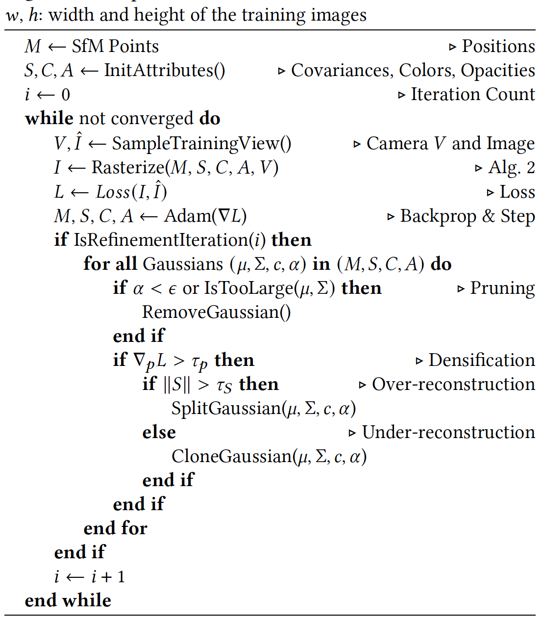
Due to the ambiguity of 3D to 2D projection, geometry may be placed incorrectly. Therefore, optimization requires the ability to create geometry and destroy or move it if it is not in the correct position. The quality of the covariance parameters of a 3D Gaussian distribution is critical to the compactness of the representation, since large uniform regions can be captured with a small number of large anisotropic Gaussian distributions.

To be able to transition from an initially sparse collection of 3D Gaussians to a denser collection that better represents the scene and has the correct parameters, the number of 3D Gaussians and their density per unit volume are controlled adaptively. The control algorithm densifies every 100 iterations and remove any Gaussians that are essentially transparent.

Fig.3 Adaptive Control of Gaussians

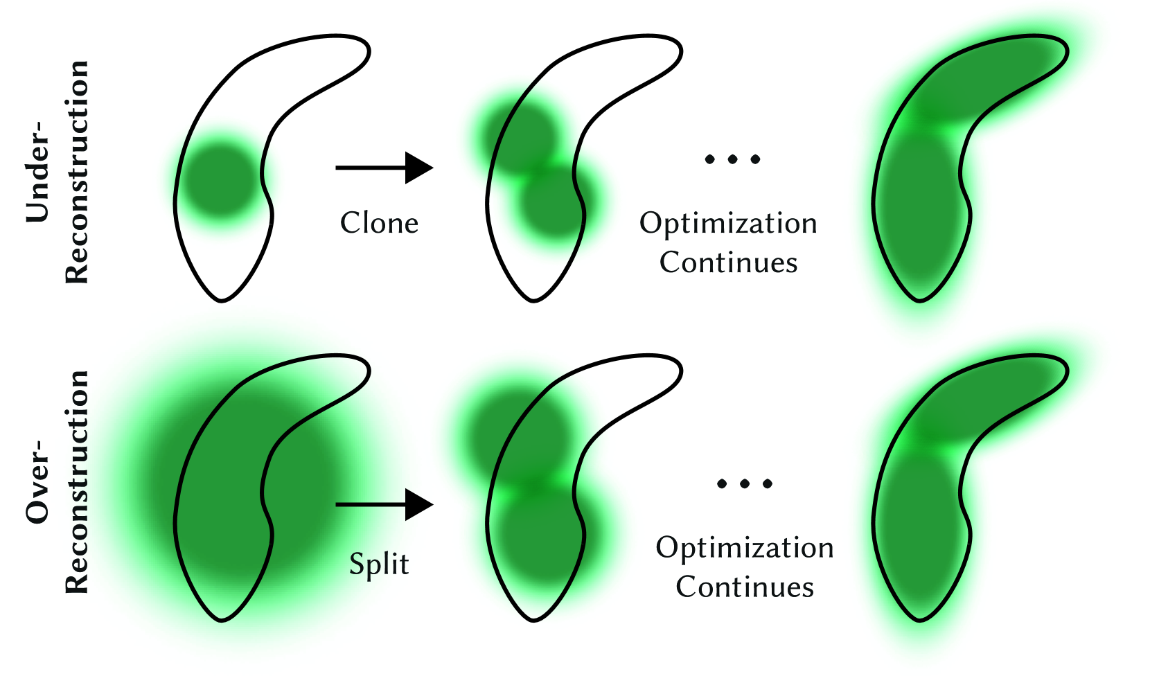
See Fig.3, for a small Gaussian in the unreconstructed region, the new geometry is created by cloning the Gaussian and moving it along the position gradient direction. Large Gaussians in regions with high variance need to be split into smaller Gaussians. Two new Gaussian distributions replace the original large Gaussian distribution, and the scaling factor is determined experimentally to divide their scales, using the original Gaussian as the sampling PDF to initialize their positions.

Floaters near the camera tend to appear during optimization, so the way to control the growth of Gaussians is to set $\alpha$ close to 0 every 3000 iterations

Optimization

A Sigmoid activation function is used to constrain $\alpha$ in the range of $[0 - 1)$ , and an exponential activation function is used for the covariance.The initial covariance matrix is estimated as an isotropic Gaussian matrix with axes equal to the mean distance to the nearest three points. The loss function is a combination of L1 and D-SSIM terms

$$
\mathcal{L} = (1 - \lambda)\mathcal{L}_1 + \lambda\mathcal{L}_{\text{D-SSIM}}
$$

Fig.4 Optimization

Reference

1. Kerbl, B., Kopanas, G., Leimkuehler, T., & Drettakis, G. (2023). 3D Gaussian Splatting for Real-Time Radiance Field Rendering. ACM Transactions on Graphics (TOG), 42, 1 - 14. ↩
2. 3D Gaussian Splatting for Real-Time Radiance Field Rendering 笔记 ↩
3. 论文简析：3D Gaussian Splatting !!! ↩
4. 3D Gaussian Splatting笔记 ↩
5. 【论文讲解】用点云结合3D高斯构建辐射场，成为快速训练、实时渲染的新SOTA！ ↩